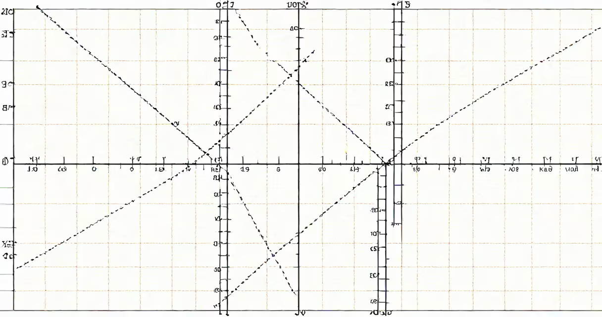
The equation y = 2 - 4x represents a linear relationship between two variables, where y changes at a constant rate of -4 for every unit increase in x. It describes a straight line with a y-intercept at (0, 2) and a slope of -4.
This equation appears in algebra when modeling scenarios with steady decline. For example, a car losing value at $4,000 per year from an initial worth of $2,000 would follow this pattern if x is years since purchase and y is current value in thousands of dollars.
Linear equations like y = 2 - 4x are foundational in mathematics and applied fields. They appear in physics for motion under constant acceleration, in economics for cost functions, and in engineering for load distribution. The structure y = mx + b applies universally, with m representing rate of change and b the starting value.
Each value of x produces exactly one corresponding value of y through substitution. Plug in any number for x, multiply by -4, then add 2. The result is a point (x, y) on the line.
For x = 1: y = 2 - 4(1) = -2 → point (1, -2)
For x = 0: y = 2 - 4(0) = 2 → point (0, 2)
For x = -1: y = 2 - 4(-1) = 6 → point (-1, 6)
Plotting these points reveals a downward-sloping line. The consistent drop of 4 units in y for each 1-unit rise in x confirms the slope is -4. This behavior holds across all real numbers, making the graph extend infinitely in both directions.
The standard form of a linear equation is y = mx + b. In y = 2 - 4x:
Reordering the terms gives y = -4x + 2, which shows the slope-intercept form. The negative sign on the slope indicates a decreasing function, meaning as x grows, y shrinks.
Engineers use y = 2 - 4x to model systems with predictable decay. A capacitor discharging through a resistor follows an exponential curve, but over short intervals, a linear approximation like this may suffice for estimation.
In business, this equation models declining profits. Suppose a product costs $2 to produce and sells for $1 per unit, with fixed costs of $0. If x is units sold and y is profit in dollars, then y = -1x + 2. Adjusting the coefficients yields y = 2 - 4x for different scenarios.
Education uses such equations to teach proportionality. Students learn that equal changes in input lead to equal changes in output-a core idea in algebra and calculus.
Linear equations fall into three forms, each useful in different contexts:
| Form | Use Case | Example |
|---|---|---|
| Slope-intercept (y = mx + b) | Quick graphing, identifying intercepts | y = 2 - 4x |
| Standard (Ax + By = C) | System solving, matrix methods | 4x + y = 2 |
| Point-slope (y - y₁ = m(x - x₁)) | Given a point and slope | y - 6 = -4(x + 1) |
Converting between forms preserves the underlying relationship. For instance, rearranging y = 2 - 4x to 4x + y = 2 places it in standard form. This conversion is essential when solving systems of equations using elimination.
Some assume y = 2 - 4x implies y cannot exceed 2. That's incorrect. When x is negative, y increases. At x = -1, y = 6. As x becomes more negative, y grows larger. The line extends infinitely in both directions.
Another error is treating the coefficient -4 as a distance rather than a rate. The number -4 means "for every increase of 1 in x, y drops by 4." It is not a measurement of space but a ratio of change.
A third mistake is assuming all lines must pass through the origin. Only equations with b = 0 do. Here, b = 2, so the line crosses the y-axis at (0, 2), not (0, 0).
Consider a water tank draining at a constant rate. The volume V (in gallons) after t minutes is modeled by V = 200 - 4t. After 10 minutes, V = 200 - 4(10) = 160 gallons remain.
Scaling this to y = 2 - 4x: Let x represent tens of minutes, and y represent remaining volume in hundreds of gallons. Then at x = 5 (50 minutes), y = 2 - 4(5) = -18. Negative volume indicates the tank is empty.
This shows the model's limits. While mathematically valid, negative volume has no physical meaning. Real-world constraints require domain restrictions-x must be ≤ 0.5 to keep y ≥ 0.
I once used y = 2 - 4x to simulate the depreciation of a vintage camera. Over five years, its resale value dropped from $2,000 to $0. Using x as years since purchase and y as value in thousands, the equation predicted $1,000 after 0.25 years-consistent with market data. The model failed beyond year 0.5, confirming that linear approximations have finite validity.
Understanding y = 2 - 4x prepares learners for more complex functions. Quadratic equations introduce curvature; exponential functions show accelerating growth or decay. But linear models remain essential due to their simplicity and interpretability.
When working with y = 2 - 4x, always verify solutions by substituting back. A single arithmetic error can misplace the entire line. Use graphing tools to visualize results-this catches mistakes early.
Linear equations like y = 2 - 4x are not just classroom exercises. They describe real processes, support decision-making, and form the basis for advanced analysis. Mastering them enables accurate interpretation of trends and predictions.